In the preceding problems, we have seen how to learn a function $f^{*}:\mathbf{x}\rightarrow\mathbf{y}$ from examples. However, when the relation between the input $\mathbf{x}$ and the label $\mathbf{y}$ is too complex to be captured by simple models, we are faced with both a generalization problem and a computational problem. Generalization becomes difficult because large models are more prone to over-fitting and optimization becomes more expensive because it takes place in a high dimensional space.
Contents
Preprocessing and feature space
A solution, instead of trying to increase model complexity, possibly at the expense of generalization and computational cost, is to create a vector of features $\Phi(\mathbf{x})=(\phi_{1}(\mathbf{x}),\dots,\phi_{K}(\mathbf{x}))$ as a pre-processing step, which are then meant to be used as input of the learning procedure. The objective of the new supervised learning problem is then to approximate the function $f^{*}:\Phi(\mathbf{x})\rightarrow\mathbf{y}$. If the features $\phi_{i}(\mathbf{x})$ extract relevant information from the raw data $\mathbf{x}$, it can result in a simplified problem which can hopefully be solved using a simple model. The feature extraction function $\Phi$ can be seen as projecting data into a feature space, i.e. representing data so as to make the euclidean distance between training examples $d_{E}(\Phi(\mathbf{x}),\Phi(\mathbf{x}’))$ more meaningful than in the input space. Figure 7 shows how such a projection can make a non linearly separable problem separable.
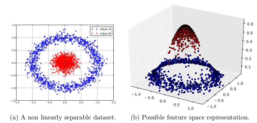
Figure 7: Illustration of the simplification power of a feature space. Given the non linearly separable classification problem (a), the projection $\Phi(x,y)=(x,y,z)$ where $z$ is a feature such that $z=\exp\left[-(x^{2}+y^{2})/2\right]$ makes the problem linearly separable in (b).
The kernel trick
In the illustration above, the projection $\Phi$ is easily computable which allows us to show the data in the feature space. However, most linear methods do not require the exact coordinates $\Phi(\mathbf{x})$ of points in the new feature space but only rely on the inner products $\left\langle \mathbf{w},\mathbf{x}\right\rangle $ between features $\mathbf{w}$ and input vectors $\mathbf{x}$. Whereas the usual inner product is taken in the input space where $\left\langle \mathbf{w},\mathbf{x}\right\rangle =\mathbf{w}^{T}\mathbf{x}$, the so called kernel trick proposes to directly define an inner product $K(\mathbf{w},\mathbf{x})$ without explicitly formulating the feature space to which it corresponds. Common choices of kernels include the polynomial kernel:
$$K(\mathbf{w},\mathbf{x})=(\mathbf{w}^{T}\mathbf{x}+c)^{d}\text{ for }d\geq0$$
and \RBF kernels, such as the Gaussian kernel:
$$K(\mathbf{w},\mathbf{x})=\exp\left[-\frac{\left\Vert \mathbf{w}-\mathbf{x}\right\Vert ^{2}}{2\sigma^{2}}\right]$$
Figure 7 can be interpreted as showing the value of the RBF kernel $K(\mathbf{x},\mathbf{0})$ corresponding to the projection of data points $\mathbf{x}$ on the zero vector in the RBF feature space.
Note that the RBF kernel corresponds to a projection into a feature space of infinite dimension which may seem counter-productive. However, high dimensional spaces make it much easier to find a linear separating surface which simplifies the problem considerably.
The manifold perspective
Under the manifold hypothesis, the data is assumed to lie on a manifold (usually low dimensional) immersed in the input space. Figure 8(a) gives a representation of a two dimensional manifold in 3D space.

Figure 8: Illustration of a two dimensional manifold immersed in 3D space (a). The same two dimensional manifold immersed in 2D space (b).
Instead of considering the coordinates of points $\mathbf{x}$ in the original input space, an interesting approach is then to try and find a feature space which recovers the structure of this manifold, i.e. to find features $\Phi(\mathbf{x})=(\phi_{1}(\mathbf{x}),\dots,\phi_{K}(\mathbf{x}))$ which correspond to the coordinates of $\mathbf{x}$ inside the manifold. This search for a good coordinate system is implicitly linked to the notion of metric. Namely, if the features $\Phi$ represent the coordinates of points inside the manifold, the Euclidean distance $\left\Vert \Phi(\mathbf{x}_{1})-\Phi(\mathbf{x}_{2})\right\Vert$ of two points in this new coordinate system should be more informative than the Euclidean distance $\left\Vert \mathbf{x}_{1}-\mathbf{x}_{2}\right\Vert$ in the input space.
Although the manifold perspective usually considers low dimensional manifolds immersed in a high dimensional space, the idea can also be applied to consider manifolds of same, or even greater, dimension than the input (unfortunately, the author was unable to make a nice figure illustrating this fact). Figure 8(b) shows how the manifold perspective can be useful to understand the impact of metrics in this setting: even though it shows a two dimensional manifold in 2D space, the Euclidean metric in the input space does not reflect the structure of the manifold, especially in the region where it folds. By using features, it may be possible to recover a more suitable coordinate system, and thus a better metric.
Unsupervised representation learning
Although the projection into a feature space can be a very powerful tool, interesting features are often found with hard work, sometimes after years of research. Nevertheless, it is sometimes possible to learn interesting features with an unsupervised algorithm, i.e. with unsupervised representation learning. Assuming a suitable set of features can be learned, the final supervised problem becomes simpler.
Putting aside the usually simple final problem, one could argue that learning representations only transforms a supervised learning problem into an equally difficult unsupervised learning problem. However, this transformation has several benefits.
Better generalization
In any practical application, the input variable $\mathbf{x}$ is expected to carry a lot of information about itself and only little information about the target variable $\mathbf{y}$. Accordingly, an unsupervised learning problem on the variable $\mathbf{x}$ has access to a lot of information during learning and is thus less prone to over-fitting than the supervised learning problem on $\mathbf{x}$ and $\mathbf{y}$. Additionally, once a representation has been obtained with unsupervised learning, the final supervised learning problem can be solved with a small number of parameters which means that over-fitting is, again, less likely.
Access to more data with semi-supervised Learning
Learning representations with an unsupervised learning algorithm has the advantage that it only depends on unlabeled data which is easily available in most settings. Because more data is available, more complex models can be learned without an adverse effect on generalization. In essence, the complete learning procedure can then leverage the information contained in an unlabeled dataset to perform better on a supervised task. This approach is known as semi-supervised learning. Formally, a semi-supervised learning problem given two datasets
$$\mathcal{D}_{L} = \{(\mathbf{x}_{1},\mathbf{y}_{1}),\dots(\mathbf{x}_{L},\mathbf{y}_{L})\}$$
and
$$\mathcal{D}_{U} = \{\mathbf{x}_{L+1},\dots,\mathbf{x}_{N}\}$$
consists in finding a function $\hat{f}$ such that $\hat{f}(\mathbf{x}_{i})\approx\mathbf{y}_{i}$ when a label is available. Figure 9 gives an illustration of the usefulness of unlabeled data to solve a supervised task.

Figure 9: Example of the influence of unlabeled data in the semi-supervised setting. The samples ($\circ$) are represented with different colors: unlabeled (white) ,class A (red), class B (blue). The unlabeled data in (a) gives a good picture of the data distribution and may allow more complex models to be learned than in (b) where there are too few samples to find a suitable separating surface.

Figure 10: Examples of sparse and distributed representations. A sparse non-distributed representation can only have one non-zero element for any input vector (left). A non-sparse distributed representation uses all variables to represent an input (center). A sparse distributed representation can use several non zero elements but must have many zeros (right).
Although it is hard to define what constitutes a good representation in general, sparse and distributed representations seem to have interesting properties and have been the subject of a lot of attention in recent years. Formally, a sparse representation is such that the feature vector $\Phi(\mathbf{x})$ contains many zeros. The sparsity is often measured with the $L_{0}$ norm which counts the number of non-zero elements. When trying to learn a representation with an unsupervised learning algorithm, sparsity can be seen as a way to impose a constraint on the hypothesis space $\mathcal{H}$, reducing the size of the search space and therefore improving generalization. Distributed representations concern the case where each input is represented by several features. Although this does not result in a reduced search space, the representation of input patterns according to several distinct attributes allows for non-local generalization. Namely, let us consider that a set of features $\Phi(\mathbf{x})=(\phi_{1}(\mathbf{x}),\dots,\phi_{K}(\mathbf{x}))$ has been obtained with an unsupervised algorithm. Even if an input $\mathbf{x}$ is not close to any training example, it may still be interpreted as an unseen combination of existing features. An illustration of sparse and distributed representations is given in Figure 10.
Interestingly, training sparse distributed representations on natural images (the so-called natural image distribution usually corresponds to images found in the outside world, i.e. images of trees, plains and lakes, but also animals, buildings, planes, boats etc) seems to result in features which have some resemblance with the neuron receptive fields of a primate’s visual cortex [Olshausen1996, Olshausen1997]. Therefore, sparse distributed representations may have (besides their theoretical benefits) the advantage of representing information in a manner similar to ours.